The Navisworks Graphics Pipeline last got a serious overhaul more then ten years ago. I want to find out how you could implement something like Navisworks with a modern pipeline. As a starting point, I’ve decided to have a look at the Nanite pipeline introduced with Unreal Engine 5.
Unreal is a mainstream games engine with a long history. It has been through the evolution from Fixed Function Pipelines, then Programmable Shaders, onto Deferred Shading and now to GPU Driven Rendering.
Nanite is particularly interesting because it’s the first time I’ve seen a games engine with a similar philosophy to Navisworks. Brian Karis, engineering fellow at Epic Games, describes their thinking in his SIGGRAPH Presentation from 2021.
Many years ago I got to see the impact that a virtual texturing system could have on an art team. How freeing it was for the artists to use giant textures wherever they wanted and not to have to worry about memory budgets. Ever since I’ve dreamt of the day where we could do the same for geometry. The impact could be even greater. No more budgets for geometry would mean no more concern over polycounts, draw calls, or memory. Without those limitations artists could directly use film quality assets without wasting any time manually optimizing for use in real-time. It’s ridiculous how much time is wasted in optimizing art content to hit framerate.
The engine source code is easily accessible. While not Open Source, the license allows you to read, build and modify the source for your own purposes. You can freely distribute any product you build using the engine (as long as any revenue you receive is below $1,000,000). In theory, this gives me a state of the art GPU rendering pipeline to experiment with.
The Nanite Pipeline

How does Nanite achieve its aim of handling whatever geometry you can throw at it? There’s nothing like the Navisworks prioritized traversal to ensure that you hit a desired framerate.
Nanite starts from the basis that there’s a fixed number of pixels on the screen, so if you’re perfectly efficient, rendering cost would be fixed for a given resolution. As far as possible, Nanite tries to ensure that you only rasterize triangles that will be visible and that you only shade fragments that will contribute to the final result.
There are three things that Nanite needs to make this work. First, using deferred shading so that only visible pixels need to be shaded during Post Processing. Second, using a dynamic LOD structure to ensure that all triangles drawn are at least pixel size. Finally, using occlusion culling to avoid drawing triangles that are hidden.
All instances including transforms, materials and at least the root of the per mesh LOD structure need to fit in GPU memory. All instances are processed by the GPU driven pipeline each frame. Which means there is a limit on the number of instances that can be used in a scene. The Nanite SIGGRAPH presentation mentions that Nanite can comfortably handle a million instances (assuming reasonable hardware). I’ve seen stress tests that get close to 10 million instances before running out of memory (32GB RAM, 11GB VRAM), while still maintaining 30 fps.
There are no limits on the size of meshes (apart from disk space to store them). Different LOD levels are streamed into memory and paged out when no longer needed. The stress test meshes have 120 thousand triangles each, for a total of around one trillion triangles.
Prepare
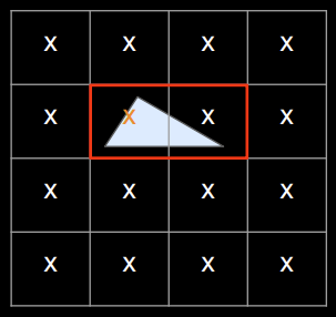
Unreal has a rich collection of utilities for scene preparation, centered around the Unreal Editor. Models can be imported from a variety of sources. Like Navisworks, complex geometry is tessellated into triangle meshes. The meshes are then further subdivided into clusters of 128 triangles or less.
SIGGRAPH 2021, A Deep Dive into Nanite Virtualized Geometry, slide 46
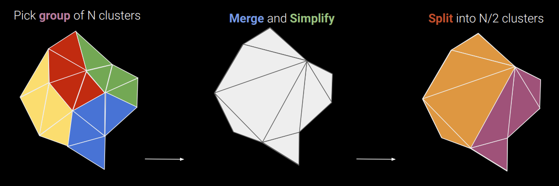
Clusters are the basis for Nanite’s LOD generation algorithm. At each LOD level, clusters are arranged into groups of 8 to 32 clusters. Each group is decimated to half the number of triangles and then split into 4 to 16 new clusters. The boundary of each group is left unchanged so that there will be no cracks when rendering adjacent clusters at LOD level L and L-1. The process repeats at the next level up with the key difference that a different set of groups with different boundaries is used. This ensures that all boundaries will eventually be decimated. The resulting clusters are organized using a bounding volume hierarchy per mesh.
LOD generation doubles the total number of triangles stored, so it is important to be as space efficient as possible. Similar to Navisworks, everything is serialized to a compressed on disk format designed so that geometry can be streamed in and decompressed on the fly.
Load
Nanite loads the scene graph, list of instances and the cluster bounding volume hierarchy for each mesh up front. Triangle clusters are loaded on demand, a group at a time, depending on the required LOD for that part of the mesh.
The on disk format is designed so that it can be efficiently decompressed using the GPU. For example, using DirectStorage on PC.
Flatten
Like all GPU Driven pipelines, Unreal maintains the entire scene (from instance list down) on the GPU. As the application modifies the scene graph, Unreal updates the GPU scene to match.
As well as having a compressed disk format, Nanite has a separate compressed in-memory format. The in-memory format is used directly for rendering so needs to have near instant decode time. Vertex attributes are quantized and bit packed. The disk representation is transcoded into the in-memory format as it is read in.
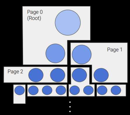
Geometry is managed within a GPU page buffer. Clusters are allocated to 128KB pages based on spatial locality and level in the LOD structure. The first page contains the top level(s) of the LOD structure and is always resident, so there is always something to render. The resident set is updated based on feedback from the Simplify stage.
Cull
Nanite performs frustum culling and occlusion culling. Occlusion culling uses a hierarchical depth buffer (HZB) with a two pass algorithm. In the first pass instances and then clusters (if the parent instance is visible) are tested against the HZB from the previous frame (using the previous frame’s transforms). The assumption is that objects that would have been visible in the last frame are highly likely to be visible in this frame. Visible clusters are rasterized. The HZB for the current frame is built based on what was just rasterized.
In the second pass, all the instances and clusters found to be occluded based on the previous HZB are retested with the current HZB and those that are now visible are rasterized. Finally, the HZB is built again ready for the next frame. In normal circumstances (camera navigating smoothly through the scene), the second pass is a small fraction of the main pass, just rasterizing those objects that became visible in the current frame.
Simplify
SIGGRAPH 2021, A Deep Dive into Nanite Virtualized Geometry, slide 27
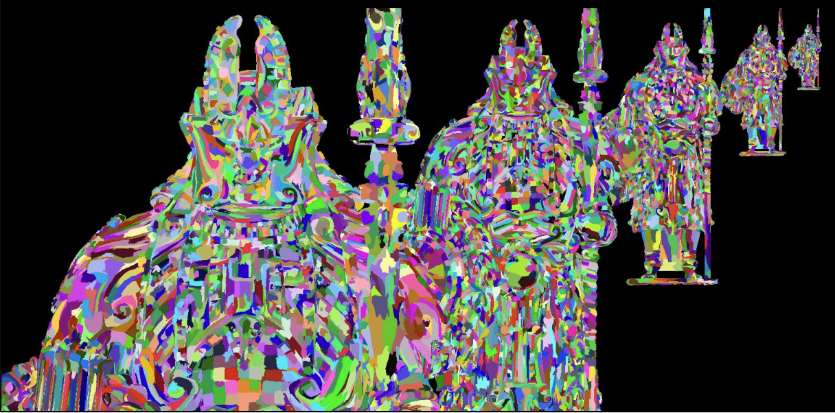
The output from the preparation phase is a set of clusters at different LOD levels. At runtime Nanite needs to select which LOD level to use for each part of each mesh. Nanite uses an error function which calculates how many pixels of error would result if a cluster at a particular LOD level is used. The error function is setup so that the error for any parent cluster (lower LOD) is higher than any of its children. This property ensures that LOD selection can be determined locally and independently (and in parallel if desired) for each cluster. A cluster should be rendered if its parent’s error is larger than a pixel and its own error is smaller than a pixel.
For efficiency there is a combined implementation for the cluster Cull and Simplify stages. The cluster BVH is traversed and at each node the HZB is tested for visibility and the LOD error function evaluated to determine whether traversal needs to continue to a more detailed LOD. Identifiers for the selected LODs are also written into an output buffer which is used by the Load-Flatten stages to update the resident set for the next frame.
Recursively traversing a tree structure using the highly parallel set of execution units provided by the GPU is an interesting problem. Nanite’s solution is to implement its own job scheduling system. It manages a GPU buffer as a queue, seeded with the root cluster for each instance. Each execution unit repeatedly reads a node from the queue, performs an occlusion and LOD selection test and then either culls the node, adds the children back into the queue or adds the clusters to a list of visible clusters to rasterize.
What happens when there are many small instances? You could end up drawing lots of sub-pixel triangles into the same pixel. This is a known limitation for Nanite.
SIGGRAPH 2021, A Deep Dive into Nanite Virtualized Geometry, slide 97
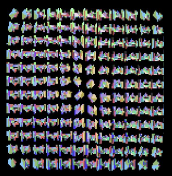
The current partial solution is to use imposters. It’s a partial solution because it only offers a constant factor improvement. Instead of drawing the 128 triangles of the root LOD, you draw a single textured quad. Nanite’s imposters consist of a texture atlas with 12x12 images (rendered from different directions) each of 12x12 pixels storing depth and triangle id. A 128 triangle cluster, where each triangle is just under pixel sized, could end up covering a 12x12 pixel square on screen.
Imposters use 40KB per mesh, which is kept resident in GPU memory. This only makes sense for large meshes and/or meshes that are frequently used. If an imposter is used, it gets rendered into the target buffer directly, bypassing vertex processing and rasterization. The appropriate image is selected depending on viewing angle, and copied into the projected rectangle in screen space, scaling and skewing the image as required.
Vertex Processing
In contrast, Vertex Processing is as simple as it gets. There are no per vertex attributes to worry about. Vertices are transformed, projected and clipped.
Rasterize
If everything is working as designed, there will be huge numbers of pixel sized triangles to rasterize. Tiny triangles are worst case for typical fixed function hardware rasterizers. Hardware rasterizers are designed to be parallel in pixels rather than triangles. They usually output in 2x2 pixel quads as that makes interpolation of vertex properties easier. There’s a lot of overhead and waste if most triangles are tiny.
Nanite includes a dedicated programmable rasterizer for clusters whose triangles are less than 32 pixels long. All 128 triangles in a cluster are processed in parallel, one per execution unit (most modern GPUs will process many clusters at the same time).
This rasterizer is three times faster on average than the hardware rasterizer for small triangles. The hardware rasterizer is still used for any clusters with large triangles. The programmable rasterizer follows the same spec for rasterization as the hardware so there are no cracks between clusters rendered using different rasterizers.
Fragment Processing
Nanite’s render target is a visibility buffer with a 64 bit atomic for each pixel. A visibility buffer stores the minimum information needed to be able to defer everything else to Post Processing. Each pixel has 30 bits for depth, 27 for visible cluster index and 7 for triangle index. Updates have to be atomic as multiple execution units could be updating the depth buffer at the same time where triangles overlap. Fragments generated from both rasterizers are written to the same visibility buffer.
Post Processing
Post Processing does a lot of heavy lifting. It needs to go from a simple visibility buffer to a final rendered scene with materials, lighting, shadows and anti-aliasing.
Material Depth Buffer
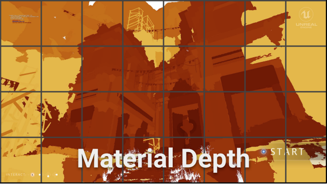
SIGGRAPH 2021, A Deep Dive into Nanite Virtualized Geometry, slide 104
The first step in Post Processing is to generate a material depth buffer. Each material is assigned a unique depth value. To generate the buffer use the visible cluster index from the visibility buffer to lookup the corresponding instance id and cluster id. Use the cluster id and triangle id from the visibility buffer to lookup a material slot id. Finally lookup the material id assigned to that material slot for this instance.
G-Buffer
The second step is to generate a G-Buffer. Nanite draws a full screen quad for each material in the scene at that material’s unique depth value. The depth test is set to “equals” so only pixels with the corresponding material id are selected. To recover the normal inputs to the material shader, Nanite adds a preamble that looks up the instance and cluster id using the visibility buffer, loads the instance transform, loads the triangle vertices, transforms them to screen space, derives barycentric coordinates for the pixel and then loads and interpolates any required vertex attributes.
A scene can have many materials so there’s potentially a huge amount of redundant work for pixels which don’t match the current material id. By using the depth test to select pixels, Nanite benefits from any early out optimizations provided by the hardware.
Many materials only cover a small portion of the screen. The full screen quad is actually drawn as a grid of tiles. Tiles that don’t contain any pixels with that material are culled in the vertex shader using a per tile bit mask built with the material depth buffer.
Lighting
Lighting is implemented with conventional deferred shading. It’s based on the same G-buffer format as the Unreal 4 engine. This allows applications to use both Nanite and the previous Unreal 4 pipeline on a per instance basis, with the two pipelines merging at the G-Buffer. Applications can easily migrate from Unreal 4 to Unreal 5 and incrementally enable Nanite for objects that will benefit from it. It also has the effect of decoupling Nanite from the lighting system which doesn’t know or care how the G-Buffer was produced.
Temporal Anti-aliasing
You may be wondering if there are “popping” artefacts due to the huge number of triangle clusters being rendered, with continual changes in LOD level as the camera moves through the scene. Nanite takes great care to ensure LOD errors are less than one pixel, which means the difference when switching between LOD levels is barely perceptible. On top of that, Unreal uses temporal anti-aliasing to blend subpixel differences over time.
Virtual Shadow Maps
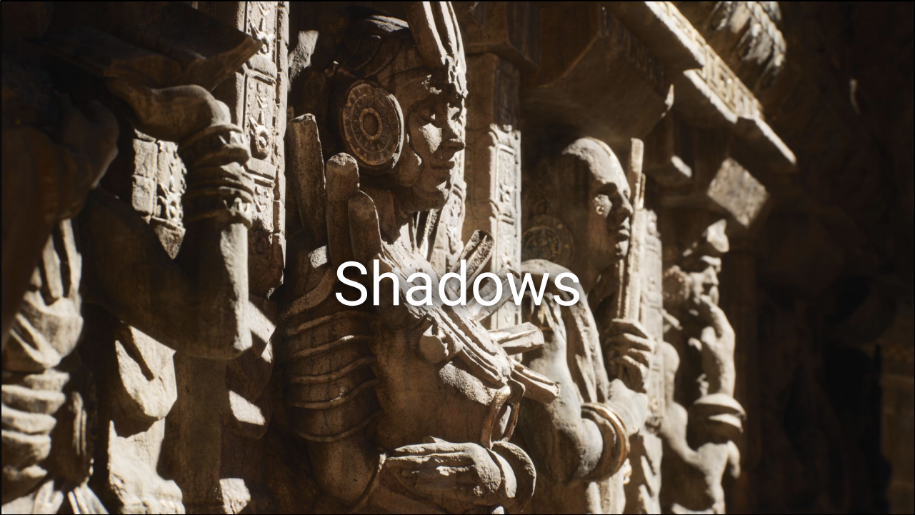
SIGGRAPH 2021, A Deep Dive into Nanite Virtualized Geometry, slide 111
Nanite enables the use of incredibly detailed, complex geometry. That means that the lighting system needs to support high resolution shadow maps to capture enough detail for accurate shadows. Unreal 5 supports virtual shadow mipmaps with up to 16k x 16k resolution. The shadow maps are virtualized and sparse. Each map is divided into pages of 128 x 128 texels, with the highest level mipmap containing 128 x 128 pages.
Pages are allocated only where needed. Each frame, the G-Buffer is processed. The engine determines the lights affecting each pixel, projects the position into shadow map space, picks the mip level where 1 texel matches the size of 1 screen pixel and marks that page in that level as needed. Pages are cached so that the only regions of the shadow map that are updated each frame are those where objects are moving or where the change in camera position brings new areas into view.
Each light may need multiple shadow maps (1 for spot lights, 6 for point lights) and multiple mipmap levels rendered. Nanite is a deep pipeline with significant per render overhead. That overhead is tiny compared to the cost of rendering the primary view. However, it would soon add up if each shadow map level was rendered separately. Instead, the Nanite pipeline supports multi-view rendering. Nanite can render all shadow maps for every light to every required mipmap level at once. For extreme scenes, this gives a 100x speedup compared to rendering each shadow map level individually.
When rendering shadow maps, Nanite performs an additional culling test. As well as testing bounding rectangles against the HZB, it also tests them against the shadow map needed pages mask. If an instance or cluster doesn’t overlap a needed page, it can be culled.
The combination of virtual shadow maps with Nanite’s rendering pipeline means that shadow cost scales roughly with screen resolution rather than scene complexity. Shadow map pages are needed where 1 texel maps to 1 pixel in the primary view. That means the number of pages and texels is proportional to screen pixels. The Nanite pipeline tries to ensure that the number of triangles rasterized to the shadow map is proportional to the number of shadow texels.
Conclusion
Nanite is hugely impressive technology. It’s going to be fascinating to see how well Nanite works with Navisworks style scenes which have huge numbers of (by Nanite standards) very simple instances.