When you’re implementing a cloud spreadsheet, it’s tempting to think of it as just another kind of database. Each row of the spreadsheet is equivalent to a row in a database. Each column in the spreadsheet is equivalent to a column in a database. Yes, spreadsheets don’t have schemas. Yes, spreadsheets can have lots of columns. However, there are plenty of examples of NoSQL databases that are schemaless and have wide column stores.
The thing that breaks the easy analogy is when you start thinking about row keys, column identifiers, insertion and deletion. Here’s the world’s most boring spreadsheet again to help focus the mind.
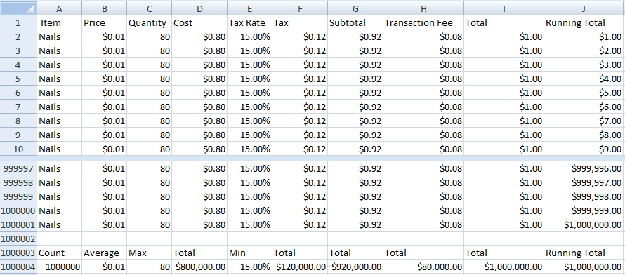
Row keys are consecutive integers. Column identifiers are alphabetical codes, effectively consecutive base 26 integers. What happens if you insert a new row at the beginning of the spreadsheet? All the other rows move down one place to make room. All the other rows now have a different row key.
What happens if you insert a new column at the beginning of the row? All the other columns move right one place to make room. All the other columns now have a different column identifier. Delete is similar with the remaining rows and columns moving the other way.
Think about what would happen if you implemented your spreadsheet as a database. Insert and Delete could result in rewriting every row in the database.
That’s ridiculous, you might think. No one would use a database this way. Give the columns meaningful identifiers rather than letters. They’re right there in the first row of your example spreadsheet. Use a value from one of the other columns as a row key, or if they’re not unique, add a GUID. Use a string if you need to support an explicit order, that way you can always come up with a new key between any pair of existing keys.
You absolutely could do that. That’s what the many Spreadsheet-Database hybrid products do. But then what you’ve built isn’t a spreadsheet anymore.
I’m building a cloud native, serverless, highly scalable spreadsheet using Event Sourcing to store the sequence of operations applied to a spreadsheet. Every so often I’ll create snapshots of the current spreadsheet state. I can then load the spreadsheet at any point in time by loading a snapshot and applying changes from that point on in the event log.
How does that work with Insert and Delete?
The rest of this post is going to build on ideas discussed in Data Structures for Spreadsheet Snapshots. You might want to refresh your memory before diving in.
Event Sourcing
Everything works very naturally with basic event sourcing. The source of truth is an event log that says an insert or delete has happened. You apply the operation to the client’s in-memory representation of the spreadsheet, which can be done simply and efficiently.
Single Segment Snapshot
Of course, event sourcing by itself isn’t enough. You need some kind of snapshot system so that you can load the state of the spreadsheet without having to replay the entire event log.

The simplest form of snapshot is one that contains the entire spreadsheet in a single segment. Again, this works very naturally with insert and delete. You load the snapshot into client memory and then apply any operations in the event log from after the snapshot was created. Inserts and deletes update the in-memory representation. To create a new snapshot, write out the in-memory representation.
Multi-Segment Snapshot
As we saw last time, maintaining single segment snapshots is an O(n2) process. To achieve reasonable efficiency you need a more complex system where each snapshot consists of multiple segments covering different parts of the event log, and where segments are shared between different snapshots.

Let’s say we’re loading snapshot 3. It consists of two segments. One created by and shared with snapshot 2 and one covering a later part of the event log created by snapshot 3.
Now things start to get interesting. What happens if there were inserts and/or deletes in the part of the event log captured by segment 3? What impact does that have on loading segment 2 and overlaying segment 3?
Let’s look at a concrete example. We have an initial event log starting to populate an empty spreadsheet.
| Event Id | Event |
|---|---|
| 1 | Set A1=Mon,C1=Wed |
| 2 | Set B2=Feb,D2=Apr |
| 3 | Set A3=2020,C3=2022 |
We then create an initial snapshot resulting in this segment.
| A | B | C | D | |
|---|---|---|---|---|
| 1 | Mon | Wed | ||
| 2 | Feb | Apr | ||
| 3 | 2020 | 2022 |
We continue with these events.
| Event Id | Event |
|---|---|
| 4 | Set B1=Tue,D1=Thu |
| 5 | Set A2=Jan,C2=Mar |
| 6 | Insert row 2 (A=Red,B=Orange,C=Yellow,D=Green) |
| 7 | Set B4=2021 |
| 8 | Delete column C |
| 9 | Set C4=2023 |
Now it’s time to create another snapshot. We write out a new segment that covers just this section of the event log and reuse the segment from the previous snapshot.
| A | B | C | |
|---|---|---|---|
| 1 | Tue | Thu | |
| 2 | Red | Orange | Green |
| 3 | Jan | ||
| 4 | 2021 | 2023 |
In theory we should be able to combine the two segments to load the complete snapshot.
| A | B | C | |
|---|---|---|---|
| 1 | Mon | Tue | Thu |
| 2 | Red | Orange | Green |
| 3 | Jan | Feb | Apr |
| 4 | 2020 | 2021 | 2023 |
But the segments don’t line up. If you overlay the second segment on top of the first you get
| A | B | C | D | |
|---|---|---|---|---|
| 1 | Mon | Tue | Thu | |
| 2 | Red | Orange | Green | Apr |
| 3 | Jan | 2022 | ||
| 4 | 2021 | 2023 |
I like to think of this problem in computer graphics terms. The segments are in different coordinate spaces. In order to combine the second segment with the first, we need to record the transform that will get the first segment into the coordinate space of the second. In our case the “transform” is just a set of rows and columns that need to be inserted and deleted. For this specific example the transform is “insert row 2, delete column C”.
When creating a snapshot we need to go back through the event log looking for all insert and delete events, combining them together to create a transform that we record with the segment we’re writing out. Redundant changes (e.g. insert row 2, delete row 2) can be removed. Lists of rows/columns can be sorted into order and combined into ranges (e.g. insert row 5-7 instead of insert 5, insert 5, insert 6).
Tiles
We want to scale to spreadsheets with millions of rows and columns which means we need to break each segment into tiles. Instead of loading complete segments, we’ll load just the tiles needed to display the required view in the client.

The view is a rectangle within the coordinate space of the most recent segment. When loading tiles from an earlier segment, we need to reverse transform the view rectangle into that segment’s coordinate space. We then use the transformed rectangle to decide which tiles to load.
To invert a transform, swap inserts and deletes. To apply the transform to a rectangle, think of what happens to the array of cells that the rectangle represents. Inserts in a row before the start of the rectangle move the rectangle down, deletes move it up. Inserts in rows in the middle of the rectangle make it bigger, deletes make it smaller.
Once we’ve identified and loaded the tiles, we forward transform each one in the same way we did for an entire segment. The contents of each tile is copied into our in-memory representation of the spreadsheet, starting from the earliest segment. Tiles from more recent segments overlay earlier tiles.
We can simplify the loading process and reduce the size of each tile by using relative addressing. Rather than storing an explicit row and column index for each cell in the tile, we store row and column relative to the top left corner of the tile. A tile can be loaded anywhere in the spreadsheet grid by adding the location of it’s top left corner to the stored row and column for each cell in the tile.
Segment Index

Conveniently, our index already stores the location of the top left corner of each tile. There’s nothing extra needed to support relative addressing.
We could also consider using relative addressing within the index itself. When using a two level row index, we can use relative addressing in the lower level index chunks. If we limit each chunk to covering at most 4 million rows, we can halve the chunk size by using 32 bit indices.
On the query and load side, nothing needs to change. We transform the view query rectangle into the segment’s coordinate space before using it to work out which tiles to load.
When writing a new segment, we need to store the transform for any dependent segment somewhere. The segment index is the obvious place to put it. This is a straight forward extension to our existing packaging ideas. We can include the transform in the same chunk as other parts of the index, or if the transform gets big enough, break it out into a separate chunk.
Just how big could a transform get? Imagine a 100 million row spreadsheet and we insert new rows between each existing row. That’s a 100 million insert ranges to store.
Encoding the Transform
The transform can be represented as four sorted lists of ranges: row inserts, row deletes, column inserts, column deletes. We can use the same principle as our row and column index to store each list. Encode each range using a pair of integers. Break the list into multiple chunks if needed.
Whether reverse transforming a query rectangle, or applying a transform to a loaded tile, we only need to use a small part of the transform. We’re interested in how many rows/columns have been inserted/deleted above and to the left of a rectangle. We only care about detailed inserts and deletes within the rectangle. Can we encode the ranges in such a way that we don’t have to iterate over them all?
Let’s look at a concrete example. We start with this simple spreadsheet.
| A | B | C | |
|---|---|---|---|
| 1 | Jan | Feb | Mar |
| 2 | Apr | May | June |
| 3 | Jul | Aug | Sep |
| 4 | Oct | Nov | Dec |
Let’s insert two rows before row 2, three rows before row 3 and one row before row 4.
| A | B | C | |
|---|---|---|---|
| 1 | Jan | Feb | Mar |
| 2 | |||
| 3 | |||
| 4 | Apr | May | June |
| 5 | |||
| 6 | |||
| 7 | |||
| 8 | Jul | Aug | Sep |
| 9 | |||
| 10 | Oct | Nov | Dec |
The simplest way of encoding the transform is like an event log. A recipe to follow.
| Index | Num |
|---|---|
| 2 | 2 |
| 5 | 3 |
| 9 | 1 |
Notice how the coordinate system is changing under our feet. Once two rows have been inserted at 2, row 3 is now row 5. Similarly, once three rows have been inserted at 5, what was originally row 4 is now row 9. This encoding makes it very difficult to do anything apart from iterate through all the steps. If I have a rectangle covering rows 3 and 4 in the original spreadsheet, the first step shifts the rectangle to (5,6), the next shifts it to (8,9) and the last expands it to (8,10).
Let’s try encoding everything in the original coordinate system. We can still iterate through this and treat it as a list of instructions by keeping track of how many rows we’ve inserted so far and adding that to the stored index.
| Index | Num |
|---|---|
| 2 | 2 |
| 3 | 3 |
| 4 | 1 |
Now I can take my (3,4) rectangle and use binary chop to find the first entry inside the rectangle. I don’t have to iterate through all the previous entries to find out that the transform makes my rectangle 1 row bigger. Unfortunately, I do need to iterate through them to find out that the transform shifts my rectangle 5 rows down.
Let’s make one more change to our encoding. Instead of storing the number of rows to insert at each index, we store the total number of rows inserted to this point. I can still determine the number of rows to insert at each step by subtracting the number stored in the previous entry.
| Index | Total Num |
|---|---|
| 2 | 2 |
| 3 | 5 |
| 4 | 6 |
As before, I can use binary chop to find the first entry (4,6) inside my rectangle. However, now the previous entry (3,5) tells me that I need to shift my rectangle by a total of 5 rows. If I’m loading a tile, I can iterate through the entries inside the tile, applying the steps needed to transform it.
If I’m transforming a query rectangle, I don’t need all the details. I only need to know how much bigger my query rectangle needs to be. I can use binary chop again to find the last entry inside the rectangle. Subtracting the first entry’s total tells me how many rows were inserted inside the rectangle.
So far we’ve considered row inserts in detail. However, a complete transform will include row deletes, column inserts and column deletes as well. Does that change anything?
Rows and columns are independent so it doesn’t matter what order we process them in. It does matter for deletes and inserts. Whichever one we process first, will change the row/column identifiers that the second depends on.
The computer graphics analogy is helpful here again. A transform goes from coordinate space A to coordinate space B and is defined in terms of coordinate space A. A subsequent transform from coordinate space B to coordinate space C has to be defined in terms of coordinate space B. As long as you apply the transforms in the correct order, everything works out as expected.
We can do the same with our insert and delete transforms. Define the order in which the transforms are applied. Let’s say Delete first, so we minimize the amount of memory used when processing. That means the Delete transform is defined using the identifiers in the source segment, but the Insert transform is defined using the identifiers as they are after Delete has been applied.
Inverting a Transform
Earlier on, I said that inverting a transform is just a matter of swapping inserts and deletes. That was a slight over simplification. A transform goes from coordinate space A to coordinate space B and is defined in terms of coordinate space A. That means the inverse transform goes from coordinate space B to coordinate space A and needs to be defined in terms of coordinate space B.
Let’s go back to our simple example. We have an insert row transform which inserts rows before row 2, 3 and 4. The inverse of that transform is a delete row transform which deletes rows starting from row 2, 5 and 9.
Converting a transform from one coordinate space to another is simple enough. Iterate through keeping hold of the total num from the previous entry. For an Insert, add that number to the current entries index. For a Delete, subtract it.
Inverting composed transforms works just like computer graphics too. Our overall transform is Delete * Insert. The inverse is Insert-1 * Delete-1. The inverse of an Insert is a Delete and vice versa, which means the result is still in the form of Delete followed by Insert.
There’s one problem with this. I came up with this funky encoding so that we could use binary chop to find just the part of the transform we’re interested in. We store the transform from one segment to another but we need to be able to transform things both ways. Inverting the transform we have, to get the one we want, means iterating through the whole thing. In which case, what’s the point of doing a fancy binary chop lookup?
The trick here is that you can do the binary chop on the original transform and invert just the entries you touch on the fly. There’s two conditions that make this possible.
- Inverting any entry is an O(1) operation. All you need is the index from the current entry and the total num from the previous entry.
- Inverting a transform doesn’t change the number of entries or the order of entries.
Coming Up
All this and I still haven’t got round to looking at segment merging. That will have to wait until next time.